Setup Analysis Conditions
Click here for instructions on how to setup and run methods.
The following information is available on this page:
Change Background Correction
- Open a worksheet.
- Select the elements.
- Click Conditions.
- Click the desired cell in the Background Correction column and then choose the desired type from the displayed list.
Click the link for more information about each type of background correction:
- None
- FittedFitted
- FACT - if you select this, 'FACT' will appear in the worksheet page navigation pane
- Off-Peak LeftOff-Peak Left
- Off-Peak RightOff-Peak Right
- Off-Peak Left+RightOff-Peak Left+Right
Change the Number of Pixels
Allows you to set how many points near the peak maximum will be used to measure the intensity of the analyte peak. The average height of these points will be denoted by the height of the 'H' marker on the spectra. If only one point is selected, this line will appear at the top of the peak.
- Open a worksheet.
- Select the elements.
- Click Conditions.
- Specify the number of pixels to be used for intensity and off-peak background correction calculations. This value will be the setting for any background correction option chosen for that wavelength.
Create and Select Condition Sets
A condition set includes measurement conditions for the wavelengths to be analyzed. Common conditions will apply to all samples and cannot be modified for individual samples, regardless of the condition set chosen. You can create up to eight condition sets.
- Open a worksheet.
- Select the elements.
- Click Conditions.
- Click the + to create up to eight different condition sets to be used on different wavelengths during the same analysis.
- Edit the measurement conditions.
- Repeat Steps 4-5 for each required condition set.
- Click the Conditions Set cell for the wavelength of interest and then select the appropriate condition set from the drop-down menu.
- To run different condition sets on the same element, add the element again on the Elements page.
Adjust Replicates
- Open a worksheet.
- Select the elements.
- Click Conditions.
- Edit the Replicates field in the Common Conditions section to set the number of times to repeat each read per solution.
All solutions will use this number of replicates. The greater number of replicates used, the better the % RSD. This will also increase the time of your sample analysis.
Adjust Custom Replicates
This feature is only available in the ICP Expert Pro feature pack.
- Open a worksheet.
- Enable Custom replicates on the Configuration page.
- Select the elements.
- Click Conditions.
- Click the
 icon next to the Replicates field.
 - Click the desired cell in the Replicates column and then enter the required number of replicates for the solution types.
- Click OK to save the changes.
Determine the Uptake Delay
The uptake delay is the length of time all solutions take to reach the plasma. If you are using an AVS 6 or 7, click here to determine the appropriate settings.

|
Hot Surfaces – Noxious Fumes – Non-Ionizing Radiation |


- Enable the AVS 4 or SVS 1.
- AVS 4: Open a worksheet and then select Autosampler and AVS 4 on the Configuration page.
- SVS 1: Click File > Options and then select Using SVS 1. Open a worksheet. Select Autosampler and SVS 1 on the Configuration page.
- Select the elements.
- Click Conditions.
- Enter an approximate uptake delay. Set the amount of time for the solution to reach the plasma.
- The ideal number will depend on the length of tube used between the sample tube and the nebulizer.
- Select whether to use the Fast pump for sample uptake and/or rinsing. If selected, the pump will run at 80 rpm unless specified otherwise.
- Using the fast pump decreases the time taken for rinsing and solution introduction.
- Turn on the plasma by clicking Plasma On or pressing the F5 key on the keyboard.
 |
The plasma will take approximately 60-80 seconds to ignite. If it fails to ignite see 'Plasma not lighting' for further information. |
 |
Tip |
- Place the sample tubing from the peristaltic pump into the wash solution and the drain tubing into the drain vessel.
- Turn on the pump to begin aspirating the solution.
- Adjust the pressure bars for even sample flow (if you have not already done so). Tell me about adjusting the pressure on the pump tubing.
- Select Signal Monitor in the View graph area to ensure you can see the results.
- Remove the sample tubing from the wash solution. Wipe the tubing and transfer it into the sample solution.
- As soon as the sample is aspirating, click the Signal Monitor button to start the wavelength scan.
- Record the time taken for the signal to stabilize after transferring the line into the sample solution.
- This should be used as the minimum uptake time. A shorter length of tubing will decrease the uptake time required.
- Click Stop.
- To export the data, right-click the graph and then select Export to export as a .csv or Microsoft Excel file.
|
If an SPS 4 is used and 'Fast pump' is enabled for the Rinse time, the rinse pump on the SPS 4 is automatically set to 'Fast' for the rinse duration. It is then changed back to the previous rate. |
Determine the Switching Valve Delay
This option only appears when the AVS 4 OR SVS 1 are enabled on the Configuration page or when 'Using SVS 1' is selected on the Options > General tab.
Enter the required switching valve delay time (the time taken for the sample solution to pass through the tubing from the autosampler to the switching valve), in seconds.
Generally, it will equal the sample uptake delay minus 2 or 3 seconds depending on the tubing length between the switching valve and nebulizer.
- Remove the connection from Port 3 on your AVS 4 or SVS 1 switching valve and place it into a beaker.
- Enable the AVS 4 or SVS 1.
- AVS 4: Open a worksheet and then select Autosampler and AVS 4 on the Configuration page.
- SVS 1: Click File > Options and then select Using SVS 1. Open a worksheet. Select Autosampler and SVS 1 on the Configuration page.
- Select the elements.
- Click Conditions.
- Enter an approximate switching valve delay.
- The ideal number will depend on the length of tube used between the switching valve and nebulizer.
- Place the sample tubing from the peristaltic pump into the rinse solution and the drain tubing into the drain vessel.
- Turn on the pump to begin aspirating the rinse solution.
- Adjust the pressure bars for even sample flow (if you have not already done so). Tell me about adjusting the pressure on the pump tubing.
- Introduce an air bubble into the line by removing and then replacing the sample line in the rinse solution.
- Record the time taken for the air bubble to travel up the line and out the end of the tubing removed from Port 3 on the valve.
- Enter the determined value in seconds into the switching valve delay field.
- Stop the pump.
- Replace the tubing into Port 3 on the valve.
Use the AVS Accessory Parameter Calculator to Determine Analysis Conditions
AVS 6 or 7 and ADS 2 only. The AVS 6/7 and ADS 2 options are only available in the ICP Expert Pro feature pack.
- Uptake pump rate (mL/min) - the rate at which the AVS pump pulls liquid through the lines during the valve uptake delay
- Inject pump rate (mL/min) - the rate at which the AVS pump pulls liquid through the lines during the stabilization delay and read time
- Valve uptake delay (s) - the length of time the AVS pump delivers the sample to the sample loop
- Bubble injection time (s) - how long argon is injected into the rinse/carrier solution liquid stream, to separate rinse/carrier and sample
- Preemptive rinse time (s) - the length of time where the autosampler probe moves from the sample tube to the rinse tube to begin rinsing the line before the uptake has finished
For example, the valve uptake delay is set at 8 seconds and the preemptive rinse time is set for 2 seconds. After 6 seconds of the valve uptake delay, the autosampler probe moves from the sample tube into the rinse tube. The total uptake time is still 8 seconds but the loop is filled with the remaining sample in the line coming from the autosampler probe. This reduces the amount of sample wasted and decreases the analysis time per sample. - Stabilization time (s) - plasma equilibration time
|
When using the AVS 6/7, the rinse time is typically set to 0. |
- Open a worksheet.
- Select Autosampler and AVS 6/7 on the Configuration page.
- Select the elements.
- Click Conditions.
- Click the calculator
 icon next to AVS Accessory to access the AVS Parameter Calculator.
- The Calculator is used to determine recommended loop volume, uptake and inject rate, uptake delay, bubble inject time, preemptive rinse time and initial stabilization delay.
- Select the peristaltic pump tubing type.
- Enter the measured length of tubing from the tip of the autosampler probe to the switching valve.
- Enter the number of tube rinses required.
- Enter the sample loop volume, if different to the recommended loop volume.
- The calculator will provide recommended times for the other parameters.
- Click Apply to copy this information to the Conditions page.
- To further optimize for the fastest analysis time, while maintaining precision, use the Optimize Analysis Time flowchart and modify the stabilization and read times.
Determine the Rinse Time
Defines the rinse time between samples and can be used with the autosampler to rinse the sample introduction system before each sample. It should be set according to your specific requirements. For manual sample introduction the user will only be asked to present the rinse solution at the completion of the run. If an autosampler is enabled, the autosampler probe will move to the rinse station and use that solution as the rinse.
|
|
Hot Surfaces – Noxious Fumes – Non-Ionizing Radiation |
To determine the rinse time:
- Open a new worksheet.
- Enable the appropriate hardware and software features.
- Select the elements.
- Click Conditions.
- Turn on the plasma by clicking Plasma On or pressing the F5 key on the keyboard.
|
The plasma will take approximately 60-80 seconds to ignite. If it fails to ignite see 'Plasma not lighting' for further information. |
|
Tip |
- Place the sample tubing from the peristaltic pump into the wash solution and the drain tubing into the drain vessel.
- Turn on the pump to begin aspirating the solution.
- Adjust the pressure bars for even sample flow (if you have not already done so). Tell me about adjusting the pressure on the pump tubing.
- Select Signal Monitor in the View graph area to ensure you can see the results.
- Remove the sample tubing from the wash solution. Wipe the tubing and transfer it into the sample solution.
- As soon as the sample is aspirating, click the Signal Monitor button to start the wavelength scan.
- Once the signal changes to indicate the sample has reached the plasma, remove the tubing from the sample solution, quickly wipe the tubing clean, and then place it into the wash solution.
- Record the time taken for the signal to stabilize after transferring the line into the wash solution. This is your rinse time.
- Click Stop.
Enable and Setup Intelligent Rinse
If enabled, an Intelligent Rinse baseline measurement takes place at the start of a worksheet (or after it is stopped and restarted) using measurement conditions from the last condition to be measured. This will measure the intensity in the rinse solution of all wavelengths which have been selected for assessment in Intelligent Rinse, regardless of which condition set they are assigned to. The baseline measurement will consist of 10 replicates of 1 second each. The baseline measurement will generate an average intensity and associated standard deviation for all wavelengths which have been selected.
After each worksheet solution is measured, Intelligent Rinse will continue to aspirate rinse solution and monitor the intensity of each of the selected lines until the measured intensities are below the threshold values (set in Washout rinse method), at which time Intelligent Rinse will stop aspirating rinse solution and the worksheet will proceed to the next solution.
This is available with ICP Expert Pro and can be used with ICP Expert with 21 CFR enabled. Intelligent Rinse is not available when dual rinse mode for the SPS 4 autosampler is selected.
To setup and enable Intelligent Rinse:
- Click File > Options > Preferences.
- Scroll to the bottom of the window and then select Enable Intelligent Rinse.
- Select the Washout rinse method.
Based on the selection, the threshold value for each wavelength is calculated by multiplying the default value of the selection (see below) by the calculated standard deviation of the Intelligent Rinse baseline measurement. If the calculated value fall below their threshold specified, the washout is finished.
- ‘Quick’ represents the fastest option and has a washout requirement of 50 standard deviations from the baseline average
- ‘Moderate’ represents a washout requirement of 20 standard deviations from the baseline average
- ‘Thorough’ represents a full rinse and has a washout requirement of 5 standard deviations from the baseline average
- Select Reacquire baseline on timeout, if required.
- If the maximum rinse time set on the Conditions page is reached before the measured intensities of all selected lines fall below their thresholds, the worksheet will proceed to the next solution. If the 'Re-acquire baseline timeout' option is enabled, an Intelligent Rinse baseline measurement will be performed before beginning measurement of the next solution. The results of this baseline measurement will then be used for subsequent Intelligent Rinse calculations.
- Click OK to close the Options window.
- Open a worksheet.
- Select the elements.
- Click Conditions.
- Select Enable Intelligent Rinse and Reacquire baseline on timeout (if required) in the Common Conditions section.
- In the Max rinse time field, specify the maximum length of rinse time before Intelligent Rinse either moves on to the next sample or re-acquires the baseline. An entry is added to the Operations Log.
- In the element table, select which elements/wavelengths to perform Intelligent Rinse.
- Select the Washout rinse method for each element/wavelength.
Enable and Select the SPS 4 or SPS 6 Rinse Port Position
Available only with the SPS 4 or SPS 6 Autosampler with dual rinse mode enabled. Intelligent Rinse is not available when dual rinse mode is selected.
To enable and select the autosampler rinse port positions:
- Click File > Options.
- Choose Agilent SPS 4 or SPS 6 from the Autosampler Model drop-down menu.
- Select Dual rinse.
- Click OK.
- Open a new worksheet.
- Ensure Autosampler is selected on the Configuration page.
- Select the elements.
- Click Conditions. Edit the desired method conditions.
- Choose the overall method Rinse Options from 1, 2, 1+2, or 2+1.
- Enter the standards information.
- If desired, select the individual solution rinse options on the Sequence page. If both rinse ports, 1+2 or 2+1, are selected, then the rinse stage of analysis will perform the full rinse duration specified in the 'Rinse time' field on the Conditions page in each rinse station.
Select the IntelliQuant Mode
Only available in IntelliQuant Screening worksheets.
Standard mode is the normal IntelliQuant measurement mode. It can take anywhere between 5-40 seconds per sample depending on the complexity of the spectral data, and can handle peaks up to around 40 million counts before over-ranging. Snapshot mode always takes around 5 seconds, but it has a more limited dynamic range and will over-range at about 1.4 million counts. Because IntelliQuant will try not to display over-ranged results, you may see different wavelengths selected as the 'best' depending on which mode is selected. To use IntelliQuant Screening during method development to help select wavelengths for use in Quantitative mode, run in 'Standard' mode.
Click here for detailed information on setting up an IntelliQuant Screening worksheet.
Perform a Signal Monitor
Signal Monitor can be performed on the Conditions page of the worksheet. Signal Monitor may be useful for monitoring the effect on signal intensity when the measurement conditions are adjusted. Adjust measurement conditions such as gas flow rates, RF power, or viewing height, etc. All common conditions are locked out while data is being collected. Using Signal Monitor is also recommended when you are setting up Sample Introduction Settings, such as Uptake time, Stabilization time and Rinse time, which are entered in the common conditions section on the Conditions page. Signal Monitor graphs for all wavelengths selected in the method are displayed as an Intensity vs Time graph.
Signal Monitor will continuously collect data for a period of 24 hours, thereafter it will maintain a rolling 24 hour period of data by removing the oldest data points. During this time you can monitor the washout time or make physical adjustments to the sample introduction system. Time resets each time Signal Monitor is reset.
|
|
Hot Surfaces – Noxious Fumes – Non-Ionizing Radiation |
To perform a Signal Monitor:
- Create a new or open an existing worksheet. Click on the Element tab.
- Select the element(s) to perform the scan on.
- Place the sample tubing from the peristaltic pump into the wash solution and the drain tubing into the drain vessel.
- Turn on the plasma by clicking Plasma On or pressing the F5 key on the keyboard.
- Turn on the pump to begin aspirating the solution.
|
The plasma will take approximately 60-80 seconds to ignite. If it fails to ignite see 'Plasma not lighting' for further information. |
|
Tip |
- Adjust the pressure bars for even sample flow (if you have not already done so). Tell me about adjusting the pressure on the pump tubing.
- Remove the sample tubing from the wash solution. Wipe the tubing and transfer it into the solution.
- Once the solution is aspirating click the Conditions tab.
|
The parameters on the Conditions page can be left at their default settings. |
- Select Signal Monitor in the View graph area to ensure you can see the results.
- Click the Signal Monitor button to start the wavelength scan.
- Click Stop to stop it.
- To export the data, right-click the graph and then select Export to export as a .csv or Microsoft Excel file.
Perform an AVS/ADS Timing Monitor Scan
The AVS/ADS Timing Monitor can be started on the Conditions page of the worksheet. As with the standard Signal Monitor, AVS/ADS Timing Monitor may be useful for monitoring the effect on signal intensity when the measurement conditions are adjusted. Adjust measurement conditions such as gas flow rates, RF power, or viewing height, etc. All common conditions are locked out while data is being collected. By watching the signal intensity as the time scan progresses, you can determine the optimal times for the AVS and ADS 2 parameters. Timing Monitor graphs for all wavelengths selected in the method are displayed as an Intensity vs Time graph.
Show me how to troubleshoot using the AVS/ADS Timing Monitor.
To perform an AVS/ADS Timing Monitor:
- Create a new or open an existing worksheet. Click on the Element tab.
- Select the element(s) to perform the monitor on.
- Turn on the plasma by clicking Plasma On or pressing the F5 key on the keyboard.
- Ensure all solutions are placed in the autosampler.
- Use the AVS/ADS Accessory calculator to determine the timing required for the AVS and ADS 2 settings.
- Enter the remaining common and measurement conditions including any condition sets required.
- Click AVS/ADS Timing Monitor.
- Select the rack and tube position for the solution used during the scan.
- Enter the autodilution factor, if required. This field is only available if the ADS 2 is enabled.
- Click Begin.
If the graph isn't displayed, select AVS/ADS Timing Monitor on the right side of the window.
- A graph is generated where a measurement is taken every 1 second.
- Measurement stops 10 seconds after the Read time of last replicate of last condition set is complete.
- The monitor is completed using all wavelengths in the worksheet and only the plasma and gas conditions from the first condition set. It also utilizes the timing from the second condition set. Plasma and gas conditions are also used for the second condition set if assigned to wavelengths in the worksheet.
- The current measurements from the graph are cleared before the new set of measurements are displayed.
- Callouts are automatically placed on the graph to indicate step changes during the measurement.
|
Tip |
The AVS/ADS Timing Monitor graph can be used to confirm a complete rinse between measurements, for troubleshooting, and to help optimize parameter times.
In the diluted solution Timing Monitor graph below, two condition sets were used on the same sample. What are the conditions used during the time scan below? Using the same ICP-OES wavelength calibration solution, a non-diluted solution Timing Monitor graph looks the same except there is less time required before the solution uptake.
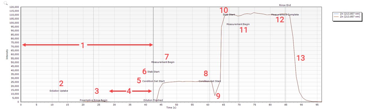
Where:
| 1. Rinsing, priming solutions and sample dilution is performed by the ADS 2. | 2. The ADS 2 is preparing for the dilution by pulling sample into the dilution loop. |
| 3. Rinsing of the ADS 2 and AVS lines begin to prevent sample contamination. | 4. Dilution occurs by mixing diluent and sample on the ADS 2 and then delivering it to the AVS sample loop and into the nebulizer and then spray chamber. |
| 5. and 6. The first condition set begins with a stabilization time to ensure sample is delivered fully into the AVS sample loop and nebulizer. The ICP Expert software has a 'built-in' stabilization time that is used along with the entered time to ensure the plasma has fully equilibrated with the diluted sample delivery. | 7. The first measurement starts. |
| 8. The measurement ends and the next condition set starts. | 9. The dip (or spike) can be caused by changing viewing modes, gas flows, and RF power. The built-in stabilization time allows the system to equilibrate after the changes occur. |
| 10. The entered stabilization starts. | 11. The next measurement begins. |
| 12. The measurement ends. | 13. Rinsing occurs. |
The conditions used for the AVS/ADS Timing Monitor above are:
Common conditions
| Common Conditions | |||
| Replicates | 3 | Pump rate - Uptake (mL/min) | 40 |
| Pump speed (rpm) | 12 | Pump rate - Inject (mL/min) | 9 |
| Rinse time (s) | 0 | Valve uptake delay | 10 |
| Fast pump | - | Bubble injection time (s) | 2 |
| Reactive dilution rinse time (s) | 0 | Preemptive rinse time | 2 |
Measurement conditions
| Measurement Conditions | |||
| Condition Set 1 | |||
| Read time (s) | 5 | Nebulizer flow (L/min) | 0.8 |
| RF power (kW) | 1.25 | Plasma flow (L/min) | 12 |
| Stabilization time (s) | 5 | Aux flow (L/min) | 1 |
| Viewing mode | Radial | Make up flow (L/min) | 0 |
| Viewing height | 8 | ||
| Condition Set 2 | |||
| Read time (s) | 5 | Nebulizer flow (L/min) | 0.6 |
| RF power (kW) | 1.35 | Plasma flow (L/min) | 12 |
| Stabilization time (s) | 3 | Aux flow (L/min) | 1 |
| Viewing mode | SVDV | Make up flow (L/min) | 0 |
| Viewing height | 9 | ||
Aqueous Versus Organic Instrument Parameters
The ICP Expert Software provides default gas and power parameters for igniting and sustaining a plasma for both aqueous and organic samples. Depending on the samples being analyzed changes may be required to maintain optimum performance and maximize torch life.
Higher Power levels coupled with lower gas flows can reduce torch life so care should be taken when selecting gas/power combinations.
 |
The combination of higher plasma power levels coupled with lower than recommended gas flows puts stresses on the torch that can substantially reduce torch life. |
The following tables show recommended operating parameters depending on the sample type being analyzed.
|
Instrument Parameters |
|
|
Nebulizer |
Glass Seaspray |
|
Spray Chamber |
Double Pass Cyclonic |
|
Torch (VDV/SVDV) |
1.8 mm Injector |
|
Torch (RV) |
1.4 mm Injector |
|
Nebulizer Gas Flow |
0.5 – 0.9 L/Min |
|
Auxiliary Gas Flow |
0.9 – 1.6 L/Min |
|
Plasma Gas Flow |
10.0 – 15.0 L/Min |
|
RF Power |
800 – 1500 Watts |
|
Instrument Parameters |
|
|
Nebulizer |
Glass Seaspray |
|
Spray Chamber |
Double Pass Cyclonic |
|
Torch |
1.4 mm Injector |
|
Nebulizer Gas Flow |
0.5 – 0.65 L/Min |
|
Auxiliary Gas Flow |
1.0 – 1.3 L/Min |
|
Plasma Gas Flow |
12.0 – 15.0 L/Min |
|
RF Power |
1300 – 1500 Watts |
Perform a Read
Performs a read of a small wavelength range around the specified element wavelength.
|
|
Hot Surfaces – Noxious Fumes – Non-Ionizing Radiation |
To perform a Read:
- Create a new or open an existing worksheet. Click on the Element tab.
- Select the element(s) to perform the read on.
- Place the sample tubing from the peristaltic pump into the wash solution and the drain tubing into the drain vessel.
- Turn on the plasma by clicking Plasma On or pressing the F5 key on the keyboard.
- Turn on the pump to begin aspirating the solution.
|
The plasma will take approximately 60-80 seconds to ignite. If it fails to ignite see 'Plasma not lighting' for further information. |
|
Tip |
- Adjust the pressure bars for even sample flow (if you have not already done so). Tell me about adjusting the pressure on the pump tubing.
- Remove the sample tubing from the wash solution. Wipe the tubing and transfer it into the solution.
- Once the solution is aspirating click the Conditions tab.
|
The parameters on the Conditions page can be left at their default settings. |
- Select Read in the View graph area to ensure you can see the results.
- Click the
 button to start the wavelength scan.
 - Click Stop to stop it.
- To export the data, right-click the graph and then select Export to export as a .csv or Microsoft Excel file.
- To overlay multiple reads, right-click the graph and select Overlay to view subsequent reads for each selected wavelength.
See also: